ModelsAirside SystemIn the airside system, models are used to describe temperature dynamics in the zones.
The dynamics of cooling a single zone or building can be represented by an energy balance. For simplicity, we considered the lumped model for the temperature of zone \(i\) as given by $$ C_i \frac{dT_i}{dt} = - H_i (T_i - T_a) - \sum_{j \neq i} \beta_{ij} (T_i - T_j) - \dot{Q}_{c,i} + \dot{Q} $$ in which \(C_i\) is the thermal capacitance of the zone, \(H_i\) is a scaled heat transfer coefficient with the ambient, \(T_a\) is the ambient temperature, \(\dot{Q}_{c,i}\) is the cooling rate from the HVAC system, \(\dot{Q}_{\mathrm{other},i}\) is an external load place on the zone, and \(\beta_{ij}\) characterizes the degree of coupling between zones \(i\) and \(j\). If zones \(i\) and \(j\) are not adjacent, then \(\beta_{ij} = 0\). Since the supervisory control system determines the zone temperature setpoints, a model is also need to relate the zone temperature setpoint \(T_{\mathrm{sp},i}\) to the cooling rate \(\dot{Q}_{c,i}\) delivered to the zone. Using an ideal proportional-integral (PI) controller, the linear cooling duty controller model is given by $$ \begin{split} \dot{Q}_{c,i} &= \dot{Q}_{\mathrm{ss},i} + K_{\mathrm{c},i} \left[ \varepsilon_i + \frac{1}{\tau_{\mathrm{I},i}} \int_0^t \varepsilon_i (t') dt' \right] \\ \varepsilon_i &= T_{\mathrm{sp},i} - T_i \\ \end{split} $$ in which \(K_{\mathrm{c},i}\) and \(\tau_{\mathrm{I},i}\) are the PI controller parameters and \(\varepsilon_i\) is the tracking error. Saturation is included as feature for airside PI due to constraints on the maximum \(\dot{Q}_{c,i}\) that is achievable. For convenience, both models can be converted to state-space form. Model parameters are available in Downloads. Waterside System\( \newcommand{\Tchws}{T_\text{CHWS}} \newcommand{\Tchwr}{T_\text{CHWR}} \newcommand{\Tcws}{T_\text{CWS}} \newcommand{\Tcwr}{T_\text{CWR}} \newcommand{\Vchw}{V_\text{CHW}} \newcommand{\Vcw}{V_\text{CW}} \newcommand{\mcw}{m_\text{CW}} \newcommand{\mair}{m_\text{air}} \newcommand{\Twb}{T_\text{WB}} \newcommand{\Qch}{Q_\text{CH}} \newcommand{\Qct}{Q_\text{CT}} \newcommand{\Wch}{W_\text{CH}} \newcommand{\Wct}{W_\text{CT}} \newcommand{\Wpump}{W_\text{P}} \newcommand{\Hhot}{H_\text{hot}} \newcommand{\Hcold}{H_\text{cold}} \newcommand{\Vhot}{V_\text{hot}} \newcommand{\Vcold}{V_\text{cold}} \newcommand{\coloneqq}{:=} \) In the waterside system, models describe equipment electricity consumption and storage tank dynamics. Equipment models are static, determining resource consumption as a function of relevant inputs for a given steady-state operating point. By contrast, storage tank models are necessarily dynamic, as storage tanks are used for time-shifting of demand.
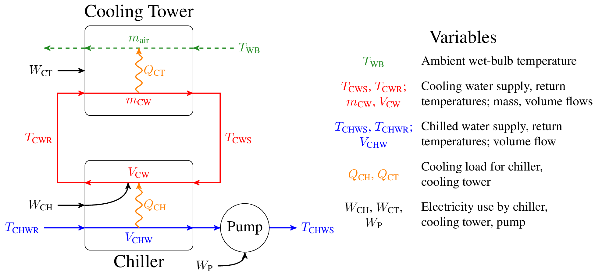
For the chilling plant used in the case study, the three types of equipment are chillers, cooling towers, and pumps. Note that the real system consists of multiple pieces of each type of equipment arranged in parallel. Each chiller is modeled using the semi-empirical Gordon-Ng model, defined below: $$ \Wch \coloneqq \left(\Qch + a_1 \Tchws + a_2 \left(1 - \frac{\Tchws}{\Tcws} \right) \right) \frac{\Tcws}{\Tchws - a_3 \Qch} - \Qch $$ The parameters \(a_1\), \(a_2\), and \(a_3\) are obtained via regression with measured data. For the purposes of optimization, the temperatures are assumed to be fixed parameters. Each cooling tower uses a a simplified effectiveness model for calculating cooling duty, with a simple cubic fit for fan electricity. $$ \begin{split} \Qct = \Qch + \Qch &\coloneqq \frac{c_1 (\mcw)^{c_3}}{1 + c_2 \left(\frac{\mcw}{\mair}\right)^{c_3}} (\Tcwr - \Twb) \label{eq:towerheat} \\ \Wct &\coloneqq \kappa (\mair)^3 \label{eq:towerfan} \end{split} $$ With fixed \(\Tcwr\) and known \(\Twb\), the first equation can be rearranged to solve for the required \(\mair\), which is then used in the second equation for electricity calculation. Coefficients \(c_1\), \(c_2\), \(c_3\), and \(\kappa\) are obtained via regression. Finally, pumps are modeled with a black-box empirical model $$ \Wpump \coloneqq b_1 \ln\left(1 + b_2 \Vchw\right) + b_3 \Vchw + b_4 $$ with regression coefficients \(b_1\) through \(b_4\). Note that the flows \(\Vcw\) and \(\mcw\) are obtained from \(\Qch\) and \(\Qct\) via the appropriate constant-heat-capacity energy balances. 
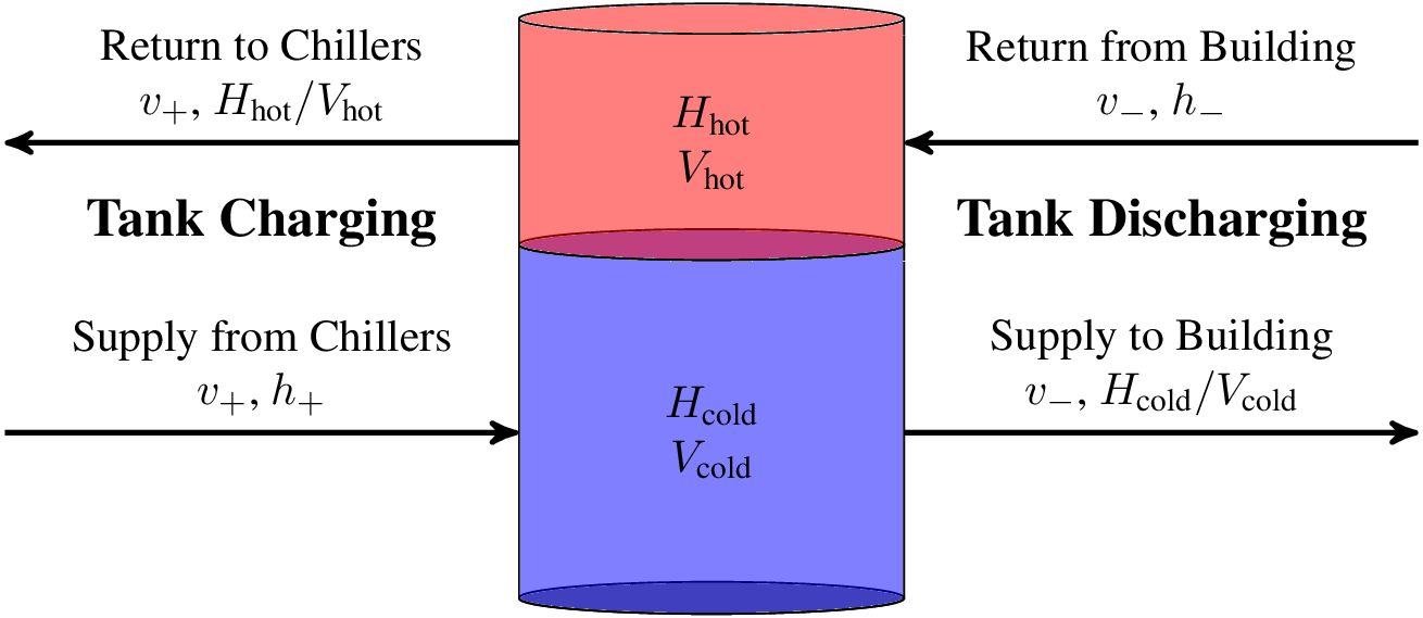
Active storage tanks are modeled using a two-layer stratified tank model. As diagrammed above, the hot and cold sections are each assumed to be uniform in temperature, with heat exchange between the two layers (proportional to the temperature difference). Total volume \(\Vhot + \Vcold\) is held constant. The dynamic model is a straightforward enthalpy balance (using known temperatures for streams entering the tank). In chilled water tanks, the main quantity of interest is the enthalpy of the cold section \(\Hcold\). For the purposes of optimization, the nonlinear tank model is replaced by a simple linear approximation of the form $$ \frac{ds}{dt} = -\sigma s + \eta \dot{Q}_\text{storage} $$ in which \(s \coloneqq \Hcold\) is the enthalpy of the cold section and \(\dot{Q}_\text{storage}\) is the rate of cold enthalpy inflow (positive) or outflow (negative). The coefficients \(\sigma\) and \(\eta\) are identified from data. Model parameters are available in Downloads. |